Week 4: Tidying up Data
Ben Best
2016-02-09 14:34
Precursors
Final Project
The instructions for your class group’s Final Project have been updated.
Schedule
The class for week 9 on March 4th conflicts with the Bren Group Project presentations, so we’ll be extending the classes before and after by 1 hour.
Invitations
organizations: invite @bbest and @naomitague to your
github.com/<org>so we can directly push to your site (vs fork & pull request)auditors: email bbest@gmail.com to ensure you get announcements via GauchoSpace
setwd()
As mentioned in wk03_dplyr, the working directory when knitting your Rmarkdown file is always the folder in which it is contained, eg for env-info/students/bbest.Rmd the working directory is env-info/students. This may be different from your R Console in RStudio which defaults to the working directory to the top level folder of your project, ie env-info. To get the two to be the same as you test code in the Console before knitting the Rmarkdown to HTML, I REQUIRE you to insert the following R chunk near the beginning (but after the Rmarkdown front matter surrounded by the rows ---) of your env-info/students/<user>.Rmd:
# set working directory if has students directory and at R Console (vs knitting)
if ('students' %in% list.files() & interactive()){
    setwd('students' )
}

# ensure working directory is students
if (basename(getwd()) != 'students'){
  stop(sprintf("WHOAH! Your working directory is not in 'students'!\n   getwd(): %s", getwd()))
}
This then ensures that “relative” paths will work the same in your R Console as when knitting your Rmarkdown to HTML. For instance:
# absolute: /Users/bbest/github/env-info/students/data/bbest_ports-bc.csv
d = read.csv('./data/bbest_ports-bc.csv')     # ./data is child of students

# absolute: /Users/bbest/github/env-info/data/r-ecology/surveys.csv
d = read.csv('../data/r-ecology/surveys.csv') # ../data is sibling of students
The first path uses this folder . since that data folder is a “child” of the students folder, whereas the second path backs up a folder .. before descending into the other data folder that is a “sibling” of the students folder.
Assignment (Individual)
For the data wrangling portion of today, append the header ## 4. Tidying up Data to your env-info/students/<user>.Rmd and include R chunks to run the demo below and give yourself the opportunity to try out possibilities with the code. Please set aside another header below this section ## 4. Answers and Tasks where you answer questions and perform tasks on applying the functions to the CO2 dataset as R chunks. Please include the question or task above the R chunk or answer.
You’ll find it easiest to copy and paste the demo portion from env-info/wk04_tidyr.Rmd but will need to understand this material enough to apply to the questions and tasks.
You will want to synchronize with ucsb-bren/env-info (ie pull request ucsb-bren/env-info to <user>/env-info, merge the pull request in <user>/env-info, and pull to update your local machine), in order to successfully knit your env-info/students/<user>.Rmd. The Rmarkdown below expects env-info/wk04_tidyr/img/data-wrangling-cheatsheet_tidyr.png and env-info/data/co2_europa.xls which are in the updated ucsb-bren/env-info.
data
The R chunks explaining the dplyr and tidyr functions below are pulled from the excellent wrangling-webinar.pdf presentation, which you should consult as you execute (see shortcuts in rstudio-IDE-cheatsheet.pdf).
EDAWR
# install.packages("devtools")
# devtools::install_github("rstudio/EDAWR")
library(EDAWR)
help(package='EDAWR')
?storms    # wind speed data for 6 hurricanes
?cases     # subset of WHO tuberculosis
?pollution # pollution data from WHO Ambient Air Pollution, 2014
?tb        # tuberculosis data
View(storms)
View(cases)
View(pollution)
slicing
# storms
storms$storm
storms$wind
storms$pressure
storms$date

# cases
cases$country
names(cases)[-1]
unlist(cases[1:3, 2:4])

# pollution
pollution$city[c(1,3,5)]
pollution$amount[c(1,3,5)]
pollution$amount[c(2,4,6)]

# ratio
storms$pressure / storms$wind
# better yet
library(dplyr)
pollution %>%
filter(city != 'New York') %>%
mutate(
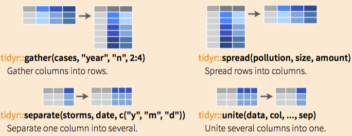
ratio = pressure / wind)tidyr
Two main functions: gather() and spread()
# install.packages("tidyr")
library(tidyr)
?gather # gather to long
?spread # spread to wide
gather
cases
gather(cases, "year", "n", 2:4)
gather(cases, "year", "n", -1)
spread
pollution
spread(pollution, size, amount)
Other functions to extract and combine columns…
separate
storms
storms2 = separate(storms, date, c("year", "month", "day"), sep = "-")
unite
storms2
unite(storms2, "date", year, month, day, sep = "-")
Recap: tidyr:
A package that reshapes the layout of data sets.
Make observations from variables with
gather()Make variables from observations withspread()Split and merge columns with
unite()andseparate()
From the data-wrangling-cheatsheet.pdf:
tidy CO2 emissions
Task. Convert the following table CO2 emissions per country since 1970 from wide to long format and output the first few rows into your Rmarkdown. I recommend consulting ?gather and you should have 3 columns in your output.
library(dplyr)
library(readxl) # install.packages('readxl')

# xls downloaded from http://edgar.jrc.ec.europa.eu/news_docs/CO2_1970-2014_dataset_of_CO2_report_2015.xls
xls = '../data/co2_europa.xls'

print(getwd())
co2 = read_excel(xls, skip=12)
co2Question. Why use skip=12 argument in read_excel()?
dplyr
A package that helps transform tabular data
# install.packages("dplyr")
library(dplyr)
?select
?filter
?arrange
?mutate
?group_by
?summarise
See sections in the data-wrangling-cheatsheet.pdf:
- Subset Variables (Columns), eg
select() - Subset Observations (Rows), eg
filter() - Reshaping Data - Change the layout of a data set, eg
arrange() - Make New Variables, eg
mutate() - Group Data, eg
group_by()andsummarise()
select
storms
select(storms, storm, pressure)
storms %>% select(storm, pressure)
filter
storms
filter(storms, wind >= 50)
storms %>% filter(wind >= 50)

storms %>%
  filter(wind >= 50) %>%
  select(storm, pressure)
mutate
storms %>%
  mutate(ratio = pressure / wind) %>%
  select(storm, ratio)
group_by
pollution
pollution %>% group_by(city)
summarise
# by city
pollution %>%
  group_by(city) %>%
  summarise(
    mean = mean(amount),
    sum = sum(amount),
    n = n())

# by size
pollution %>%
  group_by(size) %>%
  summarise(
    mean = mean(amount),
    sum = sum(amount),
    n = n())
note that summarize synonymously works
ungroup
pollution %>%
  group_by(size)

pollution %>%
  group_by(size) %>%
  ungroup()
multiple groups
tb %>%
  group_by(country, year) %>%
  summarise(cases = sum(cases))
  summarise(cases = sum(cases))
Recap: dplyr:
Extract columns with
select()and rows withfilter()Sort rows by column with
arrange()Make new columns with
mutate()Group rows by column with
group_by()andsummarise()
See sections in the data-wrangling-cheatsheet.pdf:
Subset Variables (Columns), eg
select()Subset Observations (Rows), eg
filter()Reshaping Data - Change the layout of a data set, eg
arrange()Make New Variables, eg
mutate()Group Data, eg
group_by()andsummarise()
summarize CO2 emissions
Task. Report the top 5 emitting countries (not World or EU28) for 2014 using your long format table. (You may need to convert your year column from factor to numeric, eg mutate(year = as.numeric(as.character(year))). As with most analyses, there are multiple ways to do this. I used the following additional functions: filter, arrange, desc, head).
Task. Summarize the total emissions by country (not World or EU28) across years from your long format table and return the top 5 emitting countries. (As with most analyses, there are multiple ways to do this. I used the following functions: filter, group_by, summarize, sum, arrange, desc, head).
joining data
Next week, we’ll do a bit on joining data.