joining

Precursors

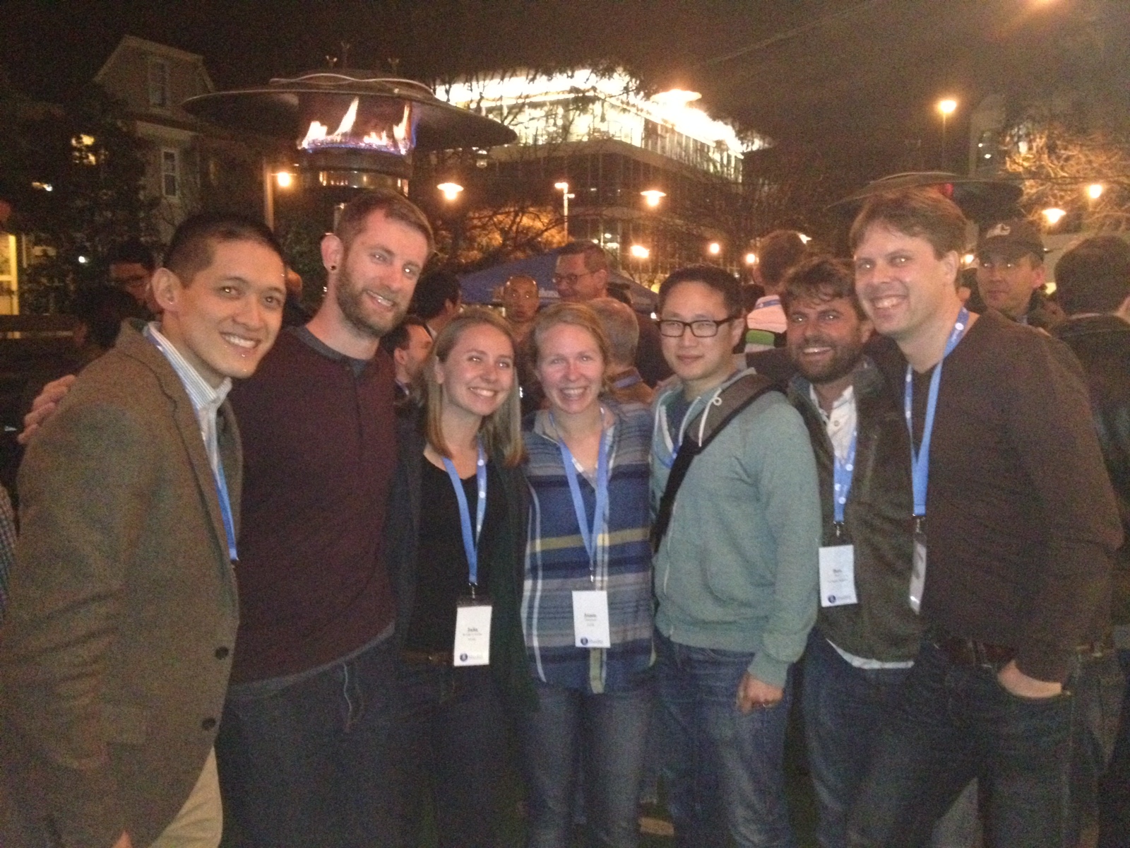
RStudio Heroes

Last weekend at 1st annual shinydevcon. Left to right, @github (affiliation):

Winston Chang @wch (RStudio)
Hadley Wickham @hadley (RStudio)
Julie Lowndes @jules32 (OHI)
Jamie Afflerbach @jafflerbach (OHI)
Joe Cheng @jcheng5 (RStudio)
Ben Best @bbest (OHI)
Herman Strop @FrissAnalytics (FrissAnalytics)

Brought some of these stickers for ya:

RStudio Shortcuts

rstudio-IDE-cheatsheet.pdf
- Show Keyboard Shortcuts ?: Alt+Shift+K (Win), Option+Shift+K (Mac)
- (Un)Comment lines #: Ctrl+Shift+C (Win), Cmd+Shift+C (Mac)
- Insert %>%: Ctrl+Shift+M (Win), Cmd+Shift+M (Mac)
- Attempt completion: Tab or Ctrl+Space (Win), Tab or Cmd+Space (Mac),
- Knit Document: Ctrl+Shift+K (Win), Cmd+Shift+K (Mac)
- Copy Lines Up/Down: Shift+Alt+$\uparrow$/$\downarrow$ (Win), Cmd+Option+$\uparrow$/$\downarrow$ (Mac)

New Assignment Github Workflow

OLD

So far to turn in individual assignments, you’ve been editing env-info/students/<user>.Rmd and knitting to env-info/students/<user>.html. Then you push to your repo <user>/env-info before submitting to the course repo ucsb-bren/env-info with a push, and pull request. To update your <user>/env-info with the latest from ucsb-bren/env-info, you also need to do an additional pull request, merge, and pull.

repo location	`<user>` permission	initialize	edit	update
`github.com/ucsb-bren/env-info`	read only		merge [BB]
`github.com/<user>/env-info`	read + write	fork	pull request	pull request , merge
`~/localdir/<user>.github.io`	read + write	clone	commit , push	pull

NEW

For future assignments, you’ll use a much simpler Github workflow with less possibilities for merge conflicts:

repo location	`<user>` permission	initialize	edit	update
`github.com/<user>/<user>.github.io`	read + write	create
`~/localdir/<user>.github.io`	read + write	clone	commit , push	pull

Similar to your class group project repo <org>/<org>.github.io which serves a web site at http://<org>.github.io, you want to initialize:

Create a repository <user>/<user>.github.io where you’ll replace <user> with your Github username (eg I created a repository bbest.github.io in which bbest is the owner). If you already have this repository created, you can simply move on. Otherwise, please also tick the box to initialize this repository with a README.
Go to Settings, Collaborators and add bbest and naomitague as collaborators. This will give us write permissions on your repository, enabling us to more easily help you fix code.
Run the equivalent of git clone http://github.com/<user>/<user>.github.io from RStudio menu File, New Project…, Version Control, Git.
Create a new folder env-info_hw inside your local repository <user>.github.io.

It is important that you use the exact spelling for all of the above. Otherwise, we won’t be able to find your homework.

Individual Assignment `wk05_ggplot`

Now, for every week’s assignment you’ll create a new Rmarkdown file inside the env-info_hw folder of your <user>.github.io repo. This week create one called wk05_ggplot.Rmd with File, New File…, R Markdown…

We’ll be able to grade assignments, because we have a roster of students by Github username, and so presume we’ll find your assignment by visiting http://<user>.github.io/env-info_hw/wk05_ggplot.html, eg http://bbest.github.io/env-info_hw/wk05_ggplot.html.

Again, it is important that you use the exact spelling above. Otherwise, we won’t be able to find your homework.

joining data

For this portion of the individual assignment, similar to last week, you’ll find it easiest to copy and paste from ## joining data onwards in env-info/wk05_joining.Rmd to your <user>.github.io/env-info_hw/wk05_ggplot.Rmd. Then you can play with different chunks of the code. Please be sure to answer all tasks and questions at the bottom.

The R chunks explaining the dplyr join functions below are pulled from the excellent wrangling-webinar.pdf presentation, which you should consult as you execute (see shortcuts in rstudio-IDE-cheatsheet.pdf).

setup

Ensure that you’re in the same working directory env-info_hw when you Knit HTML as when you test code in the Console.

wd = 'env-info_hw'

# set working directory for Console (vs Rmd)
if (wd %in% list.files() & interactive()){
    setwd(wd)
}

# ensure working directory
if (basename(getwd()) != wd){
  stop(sprintf("WHOAH! Your working directory is not in '%s'!\n   getwd(): %s", wd, getwd()))
}

`bind_cols`

bind columns between data frames

library(readr)
library(dplyr)

y = read_csv(
'x1,x2
A,1
B,2
C,3')
z = read_csv(
'x1,x2
B,2
C,3
D,4')
y
z
bind_cols(y, z)

`bind_rows`

bind rows of data frames

y
z
bind_rows(y, z)

`union`

set operation on data frames, returning all unique rows

y
z
union(y, z)

`intersect`

set operation on data frames, returning those rows in common

y
z
intersect(y, z)

`setdiff`

set operation on data frames, returning all mismatched rows

y
z
setdiff(y, z)

`left_join`

return all rows from x, and all columns from x and y. Rows in x with no match in y will have NA values in the new columns.

artists = read_csv(
'name,plays
George,sitar
John,guitar
Paul,bass
Ringo,drums')
songs = read_csv(
'song,name
Across the Universe,John
Come Together,John
"Hello, Goodbye",Paul
Peggy Sue,Buddy')
artists
songs
left_join(songs, artists, by='name')

`inner_join`

return all rows from x where there are matching values in y, and all columns from x and y

inner_join(songs, artists, by = "name")

`semi_join`

return all rows from x where there are matching values in y, keeping just columns from x

semi_join(songs, artists, by = "name")

`anti_join`

return all rows from x where there are not matching values in y, keeping just columns from x

anti_join(songs, artists, by = "name")

per capita CO₂ emissions

You’ll join the population dataset to calculate per capita CO₂ emissions.

Task. Calculate the per capita emissions by country (not World or EU28) and return the top 5 emitting countries for 2014.

Task. Summarize the per capita emissions by country (not World or EU28) as the mean (ie average) value across all years and return the top 5 emitting countries.

suppressPackageStartupMessages({
  library(readr)
  library(readxl) # install.packages('readxl')
  library(dplyr)
  library(tidyr)
  library(httr)   # install.packages('httr')
})

# co2 Excel file
url = 'http://edgar.jrc.ec.europa.eu/news_docs/CO2_1970-2014_dataset_of_CO2_report_2015.xls'
xls = 'co2_europa.xls'
if (!file.exists(xls)) writeBin(content(GET(url), 'raw'), xls)

# read in carbon dioxide emissions file
co2 = read_excel(xls, skip=12) %>%
  gather(year, ktons_co2, -Country) %>%
  filter(!Country %in% c('World','EU28') & !is.na(Country)) %>%
  mutate(year = as.integer(as.character(year))) %>%
  rename(country=Country)

## DEFINEDNAME: 21 00 00 01 0b 00 00 00 01 00 00 00 00 00 00 0d 3b 00 00 0c 00 e0 00 00 00 2c 00 
## DEFINEDNAME: 21 00 00 01 0b 00 00 00 01 00 00 00 00 00 00 0d 3b 00 00 0c 00 e0 00 00 00 2c 00 
## DEFINEDNAME: 21 00 00 01 0b 00 00 00 01 00 00 00 00 00 00 0d 3b 00 00 0c 00 e0 00 00 00 2c 00 
## DEFINEDNAME: 21 00 00 01 0b 00 00 00 01 00 00 00 00 00 00 0d 3b 00 00 0c 00 e0 00 00 00 2c 00

co2

## Source: local data frame [9,720 x 3]
## 
##                country  year    ktons_co2
##                  (chr) (int)        (dbl)
## 1          Afghanistan  1970  1813.981234
## 2              Albania  1970  4435.433037
## 3              Algeria  1970 18850.745443
## 4       American Samoa  1970     6.183023
## 5               Angola  1970  8946.495011
## 6             Anguilla  1970     2.168006
## 7  Antigua and Barbuda  1970   196.161773
## 8            Argentina  1970 87478.401090
## 9              Armenia  1970 10951.012839
## 10               Aruba  1970    40.380782
## ..                 ...   ...          ...

# read in population
popn = read_csv('https://raw.githubusercontent.com/datasets/population/master/data/population.csv') %>%
  select(country=`Country Name`, year=Year, popn=Value) 
popn

## Source: local data frame [13,484 x 3]
## 
##       country  year      popn
##         (chr) (int)     (dbl)
## 1  Arab World  1960  93485943
## 2  Arab World  1961  96058179
## 3  Arab World  1962  98728995
## 4  Arab World  1963 101496308
## 5  Arab World  1964 104359772
## 6  Arab World  1965 107318159
## 7  Arab World  1966 110379639
## 8  Arab World  1967 113543760
## 9  Arab World  1968 116787194
## 10 Arab World  1969 120078092
## ..        ...   ...       ...

In order to calculate per capita emissions, you’ll need to join the popn data frame with the co2 data frame before calculating something like ktons_co2 / popn.

One of the trickiest parts about joining data is ensuring that values in the key columns are matching. The column year is a simple 4 digit integer in both tables (after converting to as.integer() for the gathered co2). But what about country?

Let’s look at just year==2014 to see what values of country in table co2 are not found in table popn, ie anti_join():

# co2$popn not in popn$country
co2 %>%
  filter(year==2014) %>%
  anti_join(
    popn %>%
      filter(year==2014),
    by='country') %>%
  arrange(desc(ktons_co2))

## Source: local data frame [47 x 3]
## 
##                                  country  year  ktons_co2
##                                    (chr) (int)      (dbl)
## 1               United States of America  2014 5334529.74
## 2                          Int. Shipping  2014  624493.37
## 3             Iran (Islamic Republic of)  2014  618197.22
## 4                      Republic of Korea  2014  610065.60
## 5                          Int. Aviation  2014  492174.61
## 6              China, Taiwan Province of  2014  276674.74
## 7                                  Egypt  2014  225111.50
## 8     Venezuela (Bolivarian Republic of)  2014  195212.97
## 9                               Viet Nam  2014  190221.79
## 10 Democratic People s Republic of Korea  2014   59858.59
## ..                                   ...   ...        ...

Whoah, we’re missing 47 “countries”, including the “United States of America”! So what is “United States of America” called in popn$country?

# popn$country not in co2$popn
popn %>%
  filter(year==2014) %>%
  anti_join(
    co2 %>%
      filter(year==2014),
    by='country') %>%
  arrange(desc(country))

## Source: local data frame [78 x 3]
## 
##                  country  year       popn
##                    (chr) (int)      (dbl)
## 1            Yemen, Rep.  2014   24968508
## 2                  World  2014 7207735030
## 3     West Bank and Gaza  2014    4294682
## 4  Virgin Islands (U.S.)  2014     104170
## 5                Vietnam  2014   90730000
## 6          Venezuela, RB  2014   30851343
## 7    Upper middle income  2014 2354905613
## 8          United States  2014  318857056
## 9               Tanzania  2014   50757459
## 10                 Sudan  2014   38764090
## ..                   ...   ...        ...

Ok, so in popn$country we have “United States” which doesn’t get matched with “United States of America” in co2$country? How to fix this? We need a lookup table for translating country values between tables. I went ahead and made one for you by copying the two anti_join tables above and matching rows where possible.

# get lookup table to translate popn$country to co2$country
cntry = read_csv('https://raw.githubusercontent.com/ucsb-bren/env-info/gh-pages/data/co2_country_to_popn.csv')
cntry

## Source: local data frame [28 x 2]
## 
##                         country_co2         country_popn
##                               (chr)                (chr)
## 1                           Bahamas         Bahamas, The
## 2  Bolivia (Plurinational State of)              Bolivia
## 3  Democratic Republic of the Congo     Congo, Dem. Rep.
## 4                             Congo          Congo, Rep.
## 5                  C\x99te d Ivoire        Cote d'Ivoire
## 6                             Egypt     Egypt, Arab Rep.
## 7                     Faroe Islands       Faeroe Islands
## 8                            Gambia          Gambia, The
## 9              China, Hong Kong SAR Hong Kong SAR, China
## 10       Iran (Islamic Republic of)   Iran, Islamic Rep.
## ..                              ...                  ...

So before we join the tables co2 and popn, first translate country in one to match the other.

# update co2$country to popn$country
co2_m = co2 %>%
  left_join(
    cntry, 
    # note use of named vector to columns with different names
    by = c('country'='country_co2')) %>%    
  mutate(
    # note use of ifelse to upated country with popn$country_popn
    country = ifelse(!is.na(country_popn), country_popn, country))

# check that "United States of America" changed to "United States"
co2_m %>%
  filter(year==2014) %>%
  arrange(desc(country)) %>%
  head(15)

## Source: local data frame [15 x 4]
## 
##                  country  year    ktons_co2          country_popn
##                    (chr) (int)        (dbl)                 (chr)
## 1               Zimbabwe  2014 1.313540e+04                    NA
## 2                 Zambia  2014 3.367057e+03                    NA
## 3            Yemen, Rep.  2014 2.255319e+04           Yemen, Rep.
## 4         Western Sahara  2014 2.074151e+02                    NA
## 5  Virgin Islands (U.S.)  2014 1.489644e+00 Virgin Islands (U.S.)
## 6                Vietnam  2014 1.902218e+05               Vietnam
## 7          Venezuela, RB  2014 1.952130e+05         Venezuela, RB
## 8                Vanuatu  2014 1.105213e+02                    NA
## 9             Uzbekistan  2014 1.226212e+05                    NA
## 10               Uruguay  2014 8.113994e+03                    NA
## 11         United States  2014 5.334530e+06         United States
## 12        United Kingdom  2014 4.154209e+05                    NA
## 13  United Arab Emirates  2014 2.010522e+05                    NA
## 14               Ukraine  2014 2.490653e+05                    NA
## 15                Uganda  2014 4.891807e+03                    NA

Ok, so co2_m$country got updated with values to match popn$country, eg “United States of America” to “United States”.

Please use this matching co2_m to join with popn and calculate per capita emissions.

joining

Ben Best

January 29, 2016

Precursors

RStudio Heroes

RStudio Shortcuts

New Assignment Github Workflow

OLD

NEW

Individual Assignment wk05_ggplot

joining data

setup

bind_cols

bind_rows

union

intersect

setdiff

left_join

inner_join

semi_join

anti_join

per capita CO2 emissions